Real-time outbreak analysis: Ebola as a case study - part 1
Introduction
This practical (in three parts) simulates the early assessment and reconstruction of an Ebola Virus Disease (EVD) outbreak. It introduces various aspects of analysis of the early stage of an outbreak, including case fatality ratio (CFR), epicurves (part 1), growth rate estimation, contact tracing data, delays, and estimates of transmissibility (part 2), as well as transmission chain reconstruction using outbreaker2 (part 3).
Note: This practical is derived from earlier practicals called Ebola simulation part 1: early outbreak assessment and Ebola simulation part 2: outbreak reconstruction
Learning outcomes
By the end of this practical, you should be able to:
Load and clean outbreak data in R (part 1)
Estimate the case fatality ratio (CFR) (part 1)
Compute and plot incidence from linelist (part 1)
Estimate & interpret the growth rate & doubling time of the epidemic (part 2)
Estimate the serial interval from data on pairs infector / infected individuals (part 2)
Estimate & interpret the reproduction number of the epidemic (part 2)
Forecast short-term future incidence (part 2)
Reconstruct who infected whom using epidemiological and genetic data (part 3)
A novel EVD outbreak in a fictional country in West Africa
A new EVD outbreak has been notified in a fictional country in West Africa. The Ministry of Health is in charge of coordinating the outbreak response, and have contracted you as a consultant in epidemic analysis to inform the response in real time.
Required packages
The following packages, available on CRAN or github, are needed for this analysis. Install necessary packages as follows:
# install.packages("remotes")
# install.packages("readxl")
# install.packages("outbreaks")
# install.packages("incidence")
# remotes::install_github("reconhub/epicontacts@ttree")
# install.packages("distcrete")
# install.packages("epitrix")
# remotes::install_github("annecori/EpiEstim")
# remotes::install_github("reconhub/projections")
# install.packages("ggplot2")
# install.packages("magrittr")
# install.packages("binom")
# install.packages("ape")
# install.packages("outbreaker2")
# install.packages("here")Once the packages are installed, you may need to open a new R session. Then load the libraries as follows:
library(readxl)
library(outbreaks)
library(incidence)
library(epicontacts)
library(distcrete)
library(epitrix)
library(EpiEstim)
library(projections)
library(ggplot2)
library(magrittr)
library(binom)
library(ape)
library(outbreaker2)
library(here)Early data (reading data into R)
You have been given the following linelist and contact data:
linelist_20140701.xlsx: a linelist containing case information up to the 1st July 2014; and
contact_20140701.xlsx: a list of contacts reported between cases up to the 1st July 2014. “infector” indicates a potential source of infection, and “case_id” the recipient of the contact.
To read into R, download these files and use the function read_xlsx()
from the readxl package to import the data. Each import will create a
data table stored as a tibble object.
- Call the first one
linelist, and - the second one
contacts.
For instance, you first command line could look like:
linelist <- read_excel(here("data/linelist_20140701.xlsx"), na = c("", "NA"))Take some time to look at the data and structure here.
- Are the data and format similar to linelists that you have seen in the past?
- If you were part of the outbreak investigation team, what other information might you want to collect?
## [1] 169 11
## # A tibble: 6 x 11
## case_id generation date_of_infecti… date_of_onset date_of_hospita…
## <chr> <dbl> <chr> <chr> <chr>
## 1 d1fafd 0 <NA> 2014-04-07 2014-04-17
## 2 53371b 1 2014-04-09 2014-04-15 2014-04-20
## 3 f5c3d8 1 2014-04-18 2014-04-21 2014-04-25
## 4 6c286a 2 <NA> 2014-04-27 2014-04-27
## 5 0f58c4 2 2014-04-22 2014-04-26 2014-04-29
## 6 49731d 0 2014-03-19 2014-04-25 2014-05-02
## # … with 6 more variables: date_of_outcome <chr>, outcome <chr>,
## # gender <chr>, hospital <chr>, lon <dbl>, lat <dbl>
Note that for further analyses, you will need to make sure that all
dates as stored correctly as Date objects. You can do this by using
the function as.Date, for
example:
linelist$date_of_onset <- as.Date(linelist$date_of_onset, format = "%Y-%m-%d")The formatted data should then look like:
## # A tibble: 6 x 11
## case_id generation date_of_infecti… date_of_onset date_of_hospita…
## <chr> <dbl> <date> <date> <date>
## 1 d1fafd 0 NA 2014-04-07 2014-04-17
## 2 53371b 1 2014-04-09 2014-04-15 2014-04-20
## 3 f5c3d8 1 2014-04-18 2014-04-21 2014-04-25
## 4 6c286a 2 NA 2014-04-27 2014-04-27
## 5 0f58c4 2 2014-04-22 2014-04-26 2014-04-29
## 6 49731d 0 2014-03-19 2014-04-25 2014-05-02
## # … with 6 more variables: date_of_outcome <date>, outcome <chr>,
## # gender <chr>, hospital <chr>, lon <dbl>, lat <dbl>
## # A tibble: 6 x 3
## infector case_id source
## <chr> <chr> <chr>
## 1 d1fafd 53371b other
## 2 f5c3d8 0f58c4 other
## 3 0f58c4 881bd4 other
## 4 f5c3d8 d58402 other
## 5 20b688 d8a13d funeral
## 6 2ae019 a3c8b8 other
Data cleaning and descriptive analysis
Look more closely at the data contained in this linelist.
- What do you notice?
## # A tibble: 6 x 11
## case_id generation date_of_infecti… date_of_onset date_of_hospita…
## <chr> <dbl> <date> <date> <date>
## 1 d1fafd 0 NA 2014-04-07 2014-04-17
## 2 53371b 1 2014-04-09 2014-04-15 2014-04-20
## 3 f5c3d8 1 2014-04-18 2014-04-21 2014-04-25
## 4 6c286a 2 NA 2014-04-27 2014-04-27
## 5 0f58c4 2 2014-04-22 2014-04-26 2014-04-29
## 6 49731d 0 2014-03-19 2014-04-25 2014-05-02
## # … with 6 more variables: date_of_outcome <date>, outcome <chr>,
## # gender <chr>, hospital <chr>, lon <dbl>, lat <dbl>
## [1] "case_id" "generation"
## [3] "date_of_infection" "date_of_onset"
## [5] "date_of_hospitalisation" "date_of_outcome"
## [7] "outcome" "gender"
## [9] "hospital" "lon"
## [11] "lat"
You may notice that there are missing entries.
An important step in analysis is to identify any mistakes in data entry.
Although it can be difficult to assess errors in hospital names, we
would expect the date of infection to always be before the date of
symptom onset.
Clean this dataset to remove any entries with negative or 0 day incubation periods.
## identify mistakes in data entry (negative incubation period)
mistakes <-
mistakes
linelist[mistakes, ]## [1] 46 63 110
## # A tibble: 3 x 11
## case_id generation date_of_infecti… date_of_onset date_of_hospita…
## <chr> <dbl> <date> <date> <date>
## 1 3f1aaf 4 2014-05-18 2014-05-18 2014-05-25
## 2 ce9c02 5 2014-05-27 2014-05-27 2014-05-29
## 3 7.0000… 6 2014-06-10 2014-06-10 2014-06-16
## # … with 6 more variables: date_of_outcome <date>, outcome <chr>,
## # gender <chr>, hospital <chr>, lon <dbl>, lat <dbl>
Save your “cleaned” linelist as a new object: linelist_clean
linelist_clean <- linelist[-mistakes, ]What other negative dates or mistakes might you want to check if you had the full dataset?
Calculating the case fatality ratio (CFR)
Here are the number of cases by outcome status. How would you calculate the CFR from this?
table(linelist_clean$outcome, useNA = "ifany")##
## Death Recover <NA>
## 60 43 63
Think about what to do with cases whose outcome is NA?
n_dead <- sum(linelist_clean$outcome %in% "Death")
n_known_outcome <- sum(linelist_clean$outcome %in% c("Death", "Recover"))
n_all <- nrow(linelist_clean)
cfr <- n_dead / n_known_outcome
cfr_wrong <- n_dead / n_all
cfr_with_CI <- binom.confint(n_dead, n_known_outcome, method = "exact")
cfr_wrong_with_CI <- binom.confint(n_dead, n_all, method = "exact")Looking at incidence curves
The first question we want to know is simply: how bad is it?. The first step of the analysis is descriptive - we want to draw an epidemic curve or epicurve. This visualises the incidence over time by date of symptom onset.
Using the package incidence, compute the daily incidence from the
linelist_clean based on the dates of symptom onset. Store the result
in an object called i_daily; the result should look like:
i_daily## <incidence object>
## [166 cases from days 2014-04-07 to 2014-06-29]
##
## $counts: matrix with 84 rows and 1 columns
## $n: 166 cases in total
## $dates: 84 dates marking the left-side of bins
## $interval: 1 day
## $timespan: 84 days
## $cumulative: FALSE
plot(i_daily, border = "black")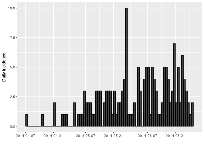
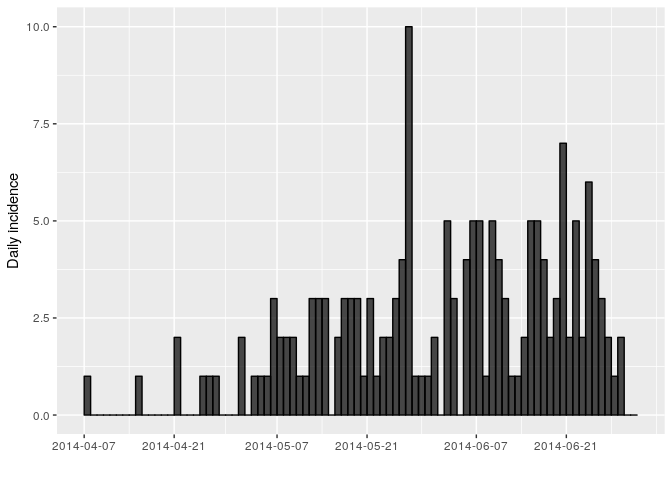
You might notice that the incidence dates i_daily$dates stops on the
last date where we have data on date of symptom onset (29th June 2014).
However close inspection of the linelist shows that the last date in the
linelist (of any entry) is in fact a bit later (1st July 2014). You can
use the argument last_date in the incidence function to change this.
## <incidence object>
## [166 cases from days 2014-04-07 to 2014-07-01]
##
## $counts: matrix with 86 rows and 1 columns
## $n: 166 cases in total
## $dates: 86 dates marking the left-side of bins
## $interval: 1 day
## $timespan: 86 days
## $cumulative: FALSE
Another issue is that it may be hard to interpret trends when looking at
daily incidence, so also compute and plot the weekly incidence
i_weekly, as follows:
i_weekly <- incidence(linelist_clean$date_of_onset, interval = 7,
last_date = as.Date(max(linelist_clean$date_of_hospitalisation, na.rm = TRUE)))
i_weekly## <incidence object>
## [166 cases from days 2014-04-07 to 2014-06-30]
## [166 cases from ISO weeks 2014-W15 to 2014-W27]
##
## $counts: matrix with 13 rows and 1 columns
## $n: 166 cases in total
## $dates: 13 dates marking the left-side of bins
## $interval: 7 days
## $timespan: 85 days
## $cumulative: FALSE
plot(i_weekly, border = "black")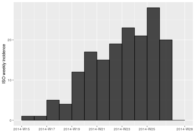
Save data and outputs
This is the end of part 1 of the practical. Before going on to part 2, you’ll need to save the following objects:
dir.create(here("data/clean")) # create clean data directory if it doesn't exist
saveRDS(i_daily, here("data/clean/i_daily.rds"))
saveRDS(i_weekly, here("data/clean/i_weekly.rds"))
saveRDS(linelist, here("data/clean/linelist.rds"))
saveRDS(linelist_clean, here("data/clean/linelist_clean.rds"))
saveRDS(contacts, here("data/clean/contacts.rds"))