Real-time outbreak analysis: Ebola as a case study - part 2
Introduction
This practical is the second (out of three) part of a practical which simulates the early assessment and reconstruction of an Ebola Virus Disease (EVD) outbreak. Please make sure you have gone through part 1 before starting part 2. In part 2 of the practical, we introduce various aspects of analysis of the early stage of an outbreak, including growth rate estimation, contact tracing data, delays, and estimates of transmissibility. Part 3 of the practical will give an introduction to transmission chain reconstruction using outbreaker2.
Note: This practical is derived from earlier practicals called Ebola simulation part 1: early outbreak assessment and Ebola simulation part 2: outbreak reconstruction
Learning outcomes
By the end of this practical (part 2), you should be able to:
Estimate & interpret the growth rate & doubling time of the epidemic
Estimate the serial interval from data on pairs infector / infected individuals
Estimate & interpret the reproduction number of the epidemic
Forecast short-term future incidence
Context: A novel EVD outbreak in a fictional country in West Africa
A new EVD outbreak has been notified in a fictional country in West Africa. The Ministry of Health is in charge of coordinating the outbreak response, and have contracted you as a consultant in epidemic analysis to inform the response in real time. You have already read in an done descriptive analysis of the data (part 1 of the practical). Now let’s do some statistical analyses!
Required packages
The following packages, available on CRAN or github, are needed for this analysis. You should have installed them in part 1 but if not, install necessary packages as follows:
# install.packages("remotes")
# install.packages("readxl")
# install.packages("outbreaks")
# install.packages("incidence")
# remotes::install_github("reconhub/epicontacts@ttree")
# install.packages("distcrete")
# install.packages("epitrix")
# remotes::install_github("annecori/EpiEstim")
# remotes::install_github("reconhub/projections")
# install.packages("ggplot2")
# install.packages("magrittr")
# install.packages("binom")
# install.packages("ape")
# install.packages("outbreaker2")
# install.packages("here")Once the packages are installed, you may need to open a new R session. Then load the libraries as follows:
library(readxl)
library(outbreaks)
library(incidence)
library(epicontacts)
library(distcrete)
library(epitrix)
library(EpiEstim)
library(projections)
library(ggplot2)
library(magrittr)
library(binom)
library(ape)
library(outbreaker2)
library(here)Read in the data processed in part 1
i_daily <- readRDS(here("data/clean/i_daily.rds"))
i_weekly <- readRDS(here("data/clean/i_weekly.rds"))
linelist <- readRDS(here("data/clean/linelist.rds"))
linelist_clean <- readRDS(here("data/clean/linelist_clean.rds"))
contacts <- readRDS(here("data/clean/contacts.rds"))Estimating the growth rate using a log-linear model
The simplest model of incidence is probably the log-linear model, i.e. a linear regression on log-transformed incidences. For this we will work with weekly incidence, to avoid having too many issues with zero incidence (which cannot be logged).
Visualise the log-transformed incidence:
ggplot(as.data.frame(i_weekly)) +
geom_point(aes(x = dates, y = log(counts))) +
scale_x_incidence(i_weekly) +
xlab("date") +
ylab("log weekly incidence") +
theme_minimal()![]()
What does this plot tell you about the epidemic?
In the incidence package, the function fit will estimate the
parameters of this model from an incidence object (here, i_weekly).
Apply it to the data and store the result in a new object called f.
You can print and use f to derive estimates of the growth rate r and
the doubling time, and add the corresponding model to the incidence
plot:
Fit a log-linear model to the weekly incidence data:
f <- incidence::fit(i_weekly)## Warning in incidence::fit(i_weekly): 1 dates with incidence of 0 ignored
## for fitting
f## <incidence_fit object>
##
## $model: regression of log-incidence over time
##
## $info: list containing the following items:
## $r (daily growth rate):
## [1] 0.04145251
##
## $r.conf (confidence interval):
## 2.5 % 97.5 %
## [1,] 0.02582225 0.05708276
##
## $doubling (doubling time in days):
## [1] 16.72148
##
## $doubling.conf (confidence interval):
## 2.5 % 97.5 %
## [1,] 12.14285 26.84302
##
## $pred: data.frame of incidence predictions (12 rows, 5 columns)
plot(i_weekly, fit = f)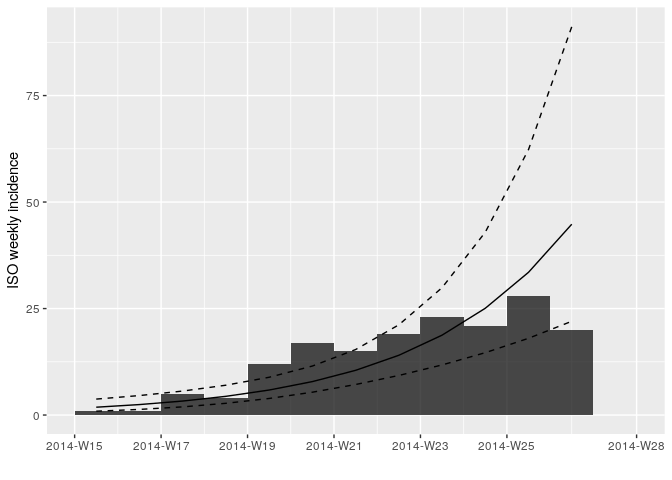
Looking at the plot and fit, do you think this is a reasonable fit?
Finding a suitable threshold date for the log-linear model, based on the observed delays
Using the plot of the log(incidence) that you plotted above, and thinking about why exponential growth may not be observed in the most recent weeks, choose a threshold date and fit the log-linear model to a suitable section of the epicurve where you think we can more reliably estimate the growth rate, r, and the doubling time.
You may want to examine how long after onset of symptoms cases are hospitalised; this may inform the threshold date you choose, as follows:
summary(as.numeric(linelist_clean$date_of_hospitalisation - linelist_clean$date_of_onset))## Min. 1st Qu. Median Mean 3rd Qu. Max.
## 0.00 1.00 2.00 3.53 5.00 22.00
# how many weeks should we discard at the end of the epicurve
n_weeks_to_discard <- min_date <- min(i_daily$dates)
max_date <- max(i_daily$dates) - n_weeks_to_discard * 7
# weekly truncated incidence
i_weekly_trunc <- subset(i_weekly,
from = min_date,
to = max_date) # discard last few weeks of data
# daily truncated incidence (not used for the linear regression but may be used later)
i_daily_trunc <- subset(i_daily,
from = min_date,
to = max_date) # remove last two weeks of dataRefit and plot your log-linear model as before but using the truncated
data i_weekly_trunc.
## <incidence_fit object>
##
## $model: regression of log-incidence over time
##
## $info: list containing the following items:
## $r (daily growth rate):
## [1] 0.04773599
##
## $r.conf (confidence interval):
## 2.5 % 97.5 %
## [1,] 0.03141233 0.06405965
##
## $doubling (doubling time in days):
## [1] 14.52043
##
## $doubling.conf (confidence interval):
## 2.5 % 97.5 %
## [1,] 10.82034 22.06609
##
## $pred: data.frame of incidence predictions (11 rows, 5 columns)
Look at the summary statistics of your fit:
summary(f$model)##
## Call:
## stats::lm(formula = log(counts) ~ dates.x, data = df)
##
## Residuals:
## Min 1Q Median 3Q Max
## -0.79781 -0.44508 -0.00138 0.35848 0.69880
##
## Coefficients:
## Estimate Std. Error t value Pr(>|t|)
## (Intercept) 0.296579 0.320461 0.925 0.379
## dates.x 0.047736 0.007216 6.615 9.75e-05 ***
## ---
## Signif. codes: 0 '***' 0.001 '**' 0.01 '*' 0.05 '.' 0.1 ' ' 1
##
## Residual standard error: 0.5298 on 9 degrees of freedom
## Multiple R-squared: 0.8294, Adjusted R-squared: 0.8105
## F-statistic: 43.76 on 1 and 9 DF, p-value: 9.754e-05
You can look at the goodness of fit (Rsquared), the estimated slope (growth rate) and the corresponding doubling time as below:
# does the model fit the data well?
adjRsq_model_fit <- summary(f$model)$adj.r.squared
# what is the estimated growth rate of the epidemic?
daily_growth_rate <- f$model$coefficients['dates.x']
# confidence interval:
daily_growth_rate_CI <- confint(f$model, 'dates.x', level=0.95)
# what is the doubling time of the epidemic?
doubling_time_days <- log(2) / daily_growth_rate
# confidence interval:
doubling_time_days_CI <- log(2) / rev(daily_growth_rate_CI)Although the log-linear is a simple and quick method for early epidemic assessment, care must be taken to only fit to the point that there is epidemic growth. Note that it may be difficult to define this point.
Contact Tracing - Looking at contacts
Contact tracing is one of the pillars of an Ebola outbreak response.
This involves identifying and following up any at risk individuals who
have had contact with a known case (i.e. may have been infected). For
Ebola, contacts are followed up for 21 days (the upper bound of the
incubation period). This ensures that contacts who become symptomatic
can be isolated quickly, reducing the chance of further transmission. We
use the full linelist here rather than linelist_clean where we
discarded entries with errors in the dates. However, the contact may
still be valid.
Using the function make_epicontacts in the epicontacts package,
create a new epicontacts object called epi_contacts. Make sure you
check the column names of the relevant to and from arguments.
epi_contacts##
## /// Epidemiological Contacts //
##
## // class: epicontacts
## // 169 cases in linelist; 60 contacts; directed
##
## // linelist
##
## # A tibble: 169 x 11
## id generation date_of_infecti… date_of_onset date_of_hospita…
## <chr> <dbl> <date> <date> <date>
## 1 d1fa… 0 NA 2014-04-07 2014-04-17
## 2 5337… 1 2014-04-09 2014-04-15 2014-04-20
## 3 f5c3… 1 2014-04-18 2014-04-21 2014-04-25
## 4 6c28… 2 NA 2014-04-27 2014-04-27
## 5 0f58… 2 2014-04-22 2014-04-26 2014-04-29
## 6 4973… 0 2014-03-19 2014-04-25 2014-05-02
## 7 f914… 3 NA 2014-05-03 2014-05-04
## 8 881b… 3 2014-04-26 2014-05-01 2014-05-05
## 9 e66f… 2 NA 2014-04-21 2014-05-06
## 10 20b6… 3 NA 2014-05-05 2014-05-06
## # … with 159 more rows, and 6 more variables: date_of_outcome <date>,
## # outcome <chr>, gender <chr>, hospital <chr>, lon <dbl>, lat <dbl>
##
## // contacts
##
## # A tibble: 60 x 3
## from to source
## <chr> <chr> <chr>
## 1 d1fafd 53371b other
## 2 f5c3d8 0f58c4 other
## 3 0f58c4 881bd4 other
## 4 f5c3d8 d58402 other
## 5 20b688 d8a13d funeral
## 6 2ae019 a3c8b8 other
## 7 20b688 974bc1 funeral
## 8 2ae019 72b905 funeral
## 9 40ae5f b8f2fd funeral
## 10 f1f60f 09e386 other
## # … with 50 more rows
You can easily plot these contacts, but with a little bit of tweaking
(see ?vis_epicontacts) you can customise for example shapes by gender
and arrow colours by source of exposure (or other variables of
interest):
# for example, look at the reported source of infection of the contacts.
table(epi_contacts$contacts$source, useNA = "ifany")##
## funeral other
## 20 40
p <- plot(epi_contacts, node_shape = "gender", shapes = c(m = "male", f = "female"), node_color = "gender", edge_color = "source", selector = FALSE)
pUsing the function match (see ?match) check that the visualised
contacts are indeed
cases.
## [1] 2 5 8 14 15 16 18 20 21 22 24 25 26 27 30 33 37
## [18] 38 40 46 48 51 58 59 62 64 68 69 70 71 73 75 79 84
## [35] 86 88 90 94 95 96 98 103 108 115 116 122 126 131 133 142 145
## [52] 146 147 148 153 155 157 160 162 166
Once you are happy that these are all indeed cases, look at the network:
- does it look like there is super-spreading (heterogeneous transmission)?
- looking at the gender of the cases, can you deduce anything from this? Are there any visible differences by gender?
Estimating transmissibility ($R$)
Branching process model
The transmissibility of the disease can be assessed through the
estimation of the reproduction number R, defined as the expected number
of secondary cases per infected case. In the early stages of an
outbreak, and assuming a large population with no immunity, this
quantity is also the basic reproduction number $R_0$, i.e. $R$ in a
large fully susceptible population.
The package EpiEstim implements a Bayesian estimation of $R$, using
dates of onset of symptoms and information on the serial interval
distribution, i.e. the distribution of time from symptom onset in a case
and symptom onset in their infector (see Cori et al., 2013, AJE 178:
1505–1512).
Briefly, EpiEstim uses a simple model describing incidence on a given
day as Poisson distributed, with a mean determined by the total force of
infection on that day:
$$ I_t ∼ Poisson(\lambda_t)$$
where $I_t$ is the incidence (based on symptom onset) on day $t$ and
$\lambda_t$ is the force of infection on that day. Noting R the
reproduction number and w() the discrete serial interval distribution,
we have:
$$\lambda_t = R \sum_{s=1}^t I_sw(t-s)$$
The likelihood (probability of observing the data given the model and parameters) is defined as a function of R:
$$L(I) = p(I|R) = \prod_{t = 1}^{T} f_P(I_t, \lambda_t)$$
where $f_P(.,\mu)$ is the probability mass function of a Poisson
distribution with mean $\mu$.
Estimating the serial interval
As data was collected on pairs of infector and infected individuals, this should be sufficient to estimate the serial interval distribution. If that was not the case, we could have used data from past outbreaks instead.
Use the function get_pairwise can be used to extract the serial
interval (i.e. the difference in date of onset between infectors and
infected individuals):
si_obs <- get_pairwise(epi_contacts, "date_of_onset")
summary(si_obs)## Min. 1st Qu. Median Mean 3rd Qu. Max.
## 1.000 5.000 6.500 9.117 12.250 30.000
## Min. 1st Qu. Median Mean 3rd Qu. Max.
## 1.000 5.000 6.500 9.117 12.250 30.000
hist(si_obs, breaks = 0:30,
xlab = "Days after symptom onset", ylab = "Frequency",
main = "Serial interval (empirical distribution)",
col = "grey", border = "white")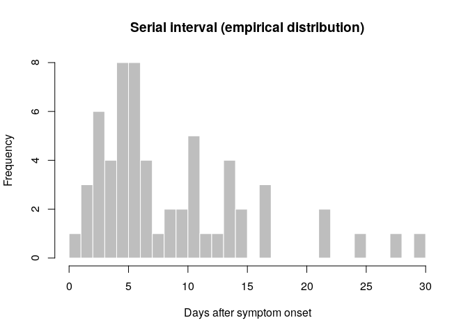
What do you think of this distribution? Make any adjustment you would
deem necessary, and then use the function fit_disc_gamma from the
package epitrix to fit a discretised Gamma distribution to these data.
Your results should approximately look like:
si_fit <- fit_disc_gamma(si_obs, w = 1)
si_fit## $mu
## [1] 8.612892
##
## $cv
## [1] 0.7277355
##
## $sd
## [1] 6.267907
##
## $ll
## [1] -183.4215
##
## $converged
## [1] TRUE
##
## $distribution
## A discrete distribution
## name: gamma
## parameters:
## shape: 1.88822148063956
## scale: 4.5613778865727
si_fit contains various information about the fitted delays, including
the estimated distribution in the $distribution slot. You can compare
this distribution to the empirical data in the following plot:
si <- si_fit$distribution
si## A discrete distribution
## name: gamma
## parameters:
## shape: 1.88822148063956
## scale: 4.5613778865727
## compare fitted distribution
hist(si_obs, xlab = "Days after symptom onset", ylab = "Frequency",
main = "Serial interval: fit to data", col = "salmon", border = "white",
50, ylim = c(0, 0.15), freq = FALSE, breaks = 0:35)
points(0:60, si$d(0:60), col = "#9933ff", pch = 20)
points(0:60, si$d(0:60), col = "#9933ff", type = "l", lty = 2)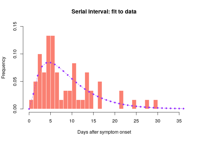
Would you trust this estimation of the generation time? How would you compare it to actual estimates from the West African EVD outbreak (WHO Ebola Response Team (2014) NEJM 371:1481–1495) with a mean of 15.3 days and a standard deviation 9.3 days?
Estimation of the Reproduction Number
Now that we have estimates of the serial interval, we can use this
information to estimate transmissibility of the disease (as measured by
$R_0$). Make sure you use a daily (not weekly) incidence object
truncated to the period where you have decided there is exponential
growth (i_daily_trunc).
Using the estimates of the mean and standard deviation of the serial
interval you just obtained, use the function estimate_R to estimate
the reproduction number (see ?estimate_R) and store the result in a
new object R.
Before using estimate_R, you need to create a config object using
the make_config function, where you will specify the time window where
you want to estimate the reproduction number as well as the mean_si
and std_si to use. For the time window, use t_start = 2 (you can
only estimate R from day 2 onwards as you are conditioning on the past
observed incidence) and specify t_end = length(i_daily_trunc$counts)
to estimate R up to the last date of your truncated incidence
i_daily_trunc.
config <- make_config(mean_si = si_fit$mu, # mean of the si distribution estimated earlier
std_si = si_fit$sd, # standard deviation of si dist estimated earlier
t_start = 2, # starting day of time window
t_end = length(i_daily_trunc$counts)) # final day of time windowR <- # use estimate_R using method = "parametric_si"
plot(R, legend = FALSE) 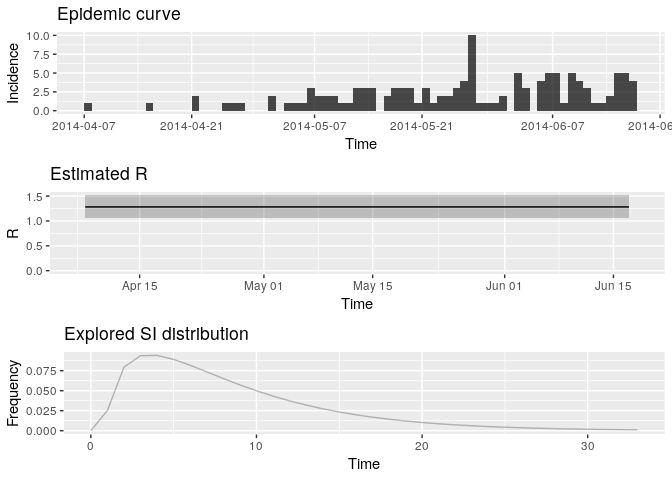
## TableGrob (3 x 1) "arrange": 3 grobs
## z cells name grob
## incid 1 (1-1,1-1) arrange gtable[layout]
## R 2 (2-2,1-1) arrange gtable[layout]
## SI 3 (3-3,1-1) arrange gtable[layout]
Extract the median and 95% credible intervals (95%CrI) for the reproduction number as follows:
R_median <- R$R$`Median(R)`
R_CrI <- c(R$R$`Quantile.0.025(R)`, R$R$`Quantile.0.975(R)`)
R_median## [1] 1.278192
R_CrI## [1] 1.068374 1.513839
Interpret these results: what do you make of the reproduction number? What does it reflect? Based on the last part of the epicurve, some colleagues suggest that incidence is going down and the outbreak may be under control. What is your opinion on this?
Note that you could have estimated R0 directly from the growth rate and
the serial interval, using the formula described in Wallinga and
Lipsitch, Proc Biol Sci, 2007: $R_0 =
\frac{1}{\int_{s=0}^{+\infty}e^{-rs}w(s)ds}$, and implemented in the
function r2R0 of the epitrix package. Although this may seem like a
complicated formula, the reasoning behind it is simple and illustrated
in the figure below: for an observed exponentially growing incidence
curve, if you know the serial interval, you can derive the reproduction
number.
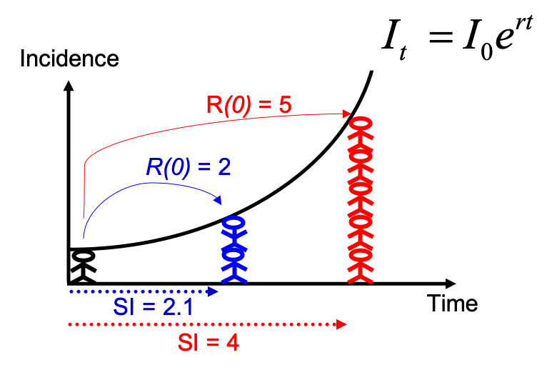
Compared to the figure above, there is uncertainty in the growth rate r, and the serial interval has a full distribution rather than a single value. This can be accounted for in estimating R as follows:
# generate a sample of R0 estimates from the growth rate and serial interval we estimated above
R_sample_from_growth_rate <- lm2R0_sample(f$model, # log-linear model which contains our estimates of the growth rate r
si$d(1:100), # serial interval distribution (truncated after 100 days)
n = 1000) # desired sample size
# plot these:
hist(R_sample_from_growth_rate)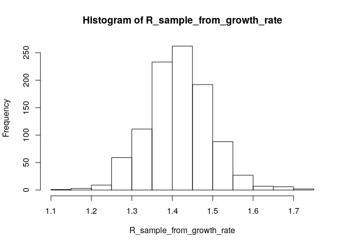
# what is the median?
R_median_from_growth_rate <- median(R_sample_from_growth_rate)
R_median_from_growth_rate # compare with R_median## [1] 1.414592
# what is the 95%CI?
R_CI_from_growth_rate <- quantile(R_sample_from_growth_rate, c(0.025, 0.975))
R_CI_from_growth_rate # compare with R_CrI## 2.5% 97.5%
## 1.266280 1.573704
Note the above estimates are slighlty different from those obtained using the branching process model. There are a few reasons for this. First, you used more detailed data (daily vs weekly incidence) for the branching process (EpiEstim) estimate. Furthermore, the log-linear model puts the same weight on all data points, whereas the branching process model puts a different weight on each data point (depending on the incidence observed at each time step). This may lead to slighlty different R estimates.
Short-term incidence forecasting
The function project from the package projections can be used to
simulate plausible epidemic trajectories by simulating daily incidence
using the same branching process as the one used to estimate $R$ in
EpiEstim. All that is needed is one, or several values of $R$ and a
serial interval distribution, stored as a distcrete object.
Here, we first illustrate how we can simulate 5 random trajectories
using a fixed value of $R$ = 1.28, the median estimate of R from
above.
Use the same daily truncated incidence object as above to simulate
future incidence.
#?project
small_proj <- project(i_daily_trunc,# incidence object
R = R_median, # R estimate to use
si = si, # serial interval distribution
n_sim = 5, # simulate 5 trajectories
n_days = 10, # over 10 days
R_fix_within = TRUE) # keep the same value of R every day
# look at each projected trajectory (as columns):
as.matrix(small_proj)## [,1] [,2] [,3] [,4] [,5]
## 2014-06-18 2 4 3 2 2
## 2014-06-19 5 4 4 4 1
## 2014-06-20 2 5 4 6 3
## 2014-06-21 6 3 3 7 2
## 2014-06-22 6 6 5 5 1
## 2014-06-23 3 2 5 2 3
## 2014-06-24 8 4 6 5 5
## 2014-06-25 7 8 1 7 5
## 2014-06-26 5 5 5 4 4
## 2014-06-27 9 9 7 7 4
Using the same principle, generate 1,000 trajectories for the next 2
weeks, using a range of plausible values of $R$.
The posterior distribution of R is gamma distributed (see Cori et
al. AJE 2013) so you can use the rgamma function to randomly draw
values from that distribution. You will also need to use the function
gamma_mucv2shapescale from the epitrix package as shown below.
sample_R <- function(R, n_sim = 1000)
{
mu <- R$R$`Mean(R)`
sigma <- R$R$`Std(R)`
Rshapescale <- gamma_mucv2shapescale(mu = mu, cv = sigma / mu)
R_sample <- rgamma(n_sim, shape = Rshapescale$shape, scale = Rshapescale$scale)
return(R_sample)
}
R_sample <- sample_R(R, 1000) # sample 1000 values of R from the posterior distribution
hist(R_sample, col = "grey") # plot histogram of sample
abline(v = R_median, col = "red") # show the median estimated R as red solid vertical line
abline(v = R_CrI, col = "red", lty = 2) # show the 95%CrI of R as red dashed vertical lines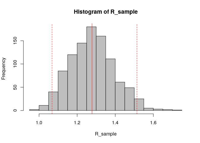
Store the results of your new projections in an object called proj.
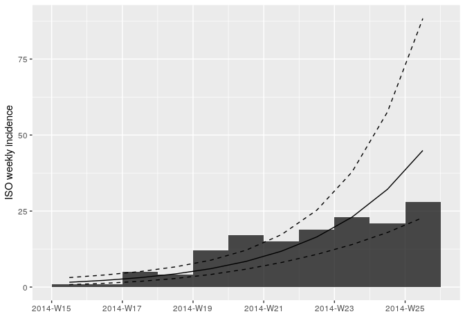
You can visualise the projections as follows:
plot(i_daily_trunc) %>% add_projections(proj, c(0.025, 0.5, 0.975))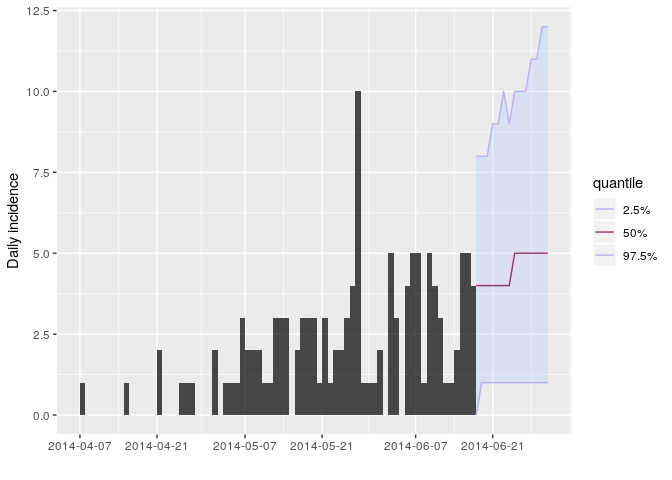
How would you interpret the following summary of the projections?
apply(proj, 1, summary)## 2014-06-18 2014-06-19 2014-06-20 2014-06-21 2014-06-22 2014-06-23
## Min. 0.000 0.000 0.000 0.00 0.000 0.000
## 1st Qu. 2.000 2.000 3.000 3.00 3.000 3.000
## Median 4.000 4.000 4.000 4.00 4.000 4.000
## Mean 3.819 3.987 4.038 4.39 4.276 4.437
## 3rd Qu. 5.000 5.000 5.000 6.00 6.000 6.000
## Max. 11.000 13.000 11.000 12.00 13.000 14.000
## 2014-06-24 2014-06-25 2014-06-26 2014-06-27 2014-06-28 2014-06-29
## Min. 0.000 0.000 0.000 0.000 0.00 0.000
## 1st Qu. 3.000 3.000 3.000 3.000 3.00 3.000
## Median 4.000 5.000 5.000 5.000 5.00 5.000
## Mean 4.528 4.866 4.909 5.095 5.28 5.351
## 3rd Qu. 6.000 6.000 7.000 7.000 7.00 7.000
## Max. 13.000 14.000 14.000 14.000 16.00 16.000
## 2014-06-30 2014-07-01
## Min. 0.000 0.000
## 1st Qu. 4.000 4.000
## Median 5.000 5.000
## Mean 5.564 5.716
## 3rd Qu. 7.000 7.000
## Max. 20.000 19.000
apply(proj, 1, function(x) mean(x > 0)) # proportion of trajectories with at least ## 2014-06-18 2014-06-19 2014-06-20 2014-06-21 2014-06-22 2014-06-23
## 0.970 0.979 0.980 0.990 0.983 0.986
## 2014-06-24 2014-06-25 2014-06-26 2014-06-27 2014-06-28 2014-06-29
## 0.993 0.993 0.989 0.988 0.995 0.987
## 2014-06-30 2014-07-01
## 0.987 0.992
# one case on each given day
apply(proj, 1, mean) # mean daily number of cases ## 2014-06-18 2014-06-19 2014-06-20 2014-06-21 2014-06-22 2014-06-23
## 3.819 3.987 4.038 4.390 4.276 4.437
## 2014-06-24 2014-06-25 2014-06-26 2014-06-27 2014-06-28 2014-06-29
## 4.528 4.866 4.909 5.095 5.280 5.351
## 2014-06-30 2014-07-01
## 5.564 5.716
apply(apply(proj, 2, cumsum), 1, summary) # projected cumulative number of cases in ## 2014-06-18 2014-06-19 2014-06-20 2014-06-21 2014-06-22 2014-06-23
## Min. 0.000 0.000 2.000 5.000 7.00 8.000
## 1st Qu. 2.000 6.000 9.000 13.000 17.00 21.000
## Median 4.000 7.000 12.000 16.000 20.00 25.000
## Mean 3.819 7.806 11.844 16.234 20.51 24.947
## 3rd Qu. 5.000 10.000 14.000 19.000 24.00 29.000
## Max. 11.000 18.000 24.000 36.000 43.00 53.000
## 2014-06-24 2014-06-25 2014-06-26 2014-06-27 2014-06-28 2014-06-29
## Min. 11.000 13.000 16.00 16.000 17.000 18.000
## 1st Qu. 24.000 28.000 32.00 37.000 41.000 45.000
## Median 29.000 34.000 39.00 44.000 49.000 54.000
## Mean 29.475 34.341 39.25 44.345 49.625 54.976
## 3rd Qu. 34.000 40.000 45.00 51.000 57.000 64.000
## Max. 60.000 69.000 83.00 94.000 105.000 116.000
## 2014-06-30 2014-07-01
## Min. 20.00 21.000
## 1st Qu. 50.00 54.000
## Median 59.00 65.000
## Mean 60.54 66.256
## 3rd Qu. 70.00 76.000
## Max. 132.00 142.000
# the next two weeksAccording to these results, what are the chances that more cases will
appear in the near future? Is this outbreak being brought under control?
Would you recommend scaling up / down the response? Is this consistent
with your estimate of $R$?
Pause !
Please let a demonstrator know when you have reached this point before proceeding further.
Accounting for uncertainty in the serial interval estimates when estimating the reproduction number
Note that this section is independent from the following ones, please skip if you don’thave time.
EpiEstim allows to explicitly account for the uncertainty in the serial interval estimates because of limited sample size of pairs of infector/infected individuals. Note that it also allows accounting for uncertainty on the dates of symptom onset for each of these pairs (which is not needed here).
Use the method = "si_from_data" option in estimate_R. To use this
option, you need to create a data frame with 4 columns: EL, ER, SL
and SR for the left (L) and right ® bounds of the observed time of
symptoms in the infector (E) and infected (S for secondary) cases. Here
we derive this from si_obs as follows:
si_data <- data.frame(EL = rep(0L, length(si_obs)),
ER = rep(1L, length(si_obs)),
SL = si_obs, SR = si_obs + 1L)We can then feed this into estimate_R (but this will take some time to
run as it estimates the serial interval distribution using an MCMC and
fully accounts for the uncertainty in the serial interval to estimate
the reproduction number).
config <- make_config(t_start = 2,
t_end = length(i_daily_trunc$counts))
R_variableSI <- estimate_R(i_daily_trunc, method = "si_from_data",
si_data = si_data,
config = config)## Running 8000 MCMC iterations
## MCMCmetrop1R iteration 1 of 8000
## function value = -186.93263
## theta =
## 0.61048
## 1.53754
## Metropolis acceptance rate = 1.00000
##
## MCMCmetrop1R iteration 1001 of 8000
## function value = -187.66955
## theta =
## 0.60839
## 1.72039
## Metropolis acceptance rate = 0.55145
##
## MCMCmetrop1R iteration 2001 of 8000
## function value = -186.33760
## theta =
## 0.84673
## 1.39242
## Metropolis acceptance rate = 0.56322
##
## MCMCmetrop1R iteration 3001 of 8000
## function value = -186.84716
## theta =
## 0.95161
## 1.19723
## Metropolis acceptance rate = 0.56448
##
## MCMCmetrop1R iteration 4001 of 8000
## function value = -187.56424
## theta =
## 0.86940
## 1.46982
## Metropolis acceptance rate = 0.55711
##
## MCMCmetrop1R iteration 5001 of 8000
## function value = -186.49130
## theta =
## 0.76777
## 1.49876
## Metropolis acceptance rate = 0.55449
##
## MCMCmetrop1R iteration 6001 of 8000
## function value = -186.49278
## theta =
## 0.86552
## 1.39227
## Metropolis acceptance rate = 0.55257
##
## MCMCmetrop1R iteration 7001 of 8000
## function value = -186.98037
## theta =
## 1.00900
## 1.19664
## Metropolis acceptance rate = 0.55092
##
##
##
## @@@@@@@@@@@@@@@@@@@@@@@@@@@@@@@@@@@@@@@@@@@@@@@@@@@@@@@@@
## The Metropolis acceptance rate was 0.55012
## @@@@@@@@@@@@@@@@@@@@@@@@@@@@@@@@@@@@@@@@@@@@@@@@@@@@@@@@@
##
## Gelman-Rubin MCMC convergence diagnostic was successful.
##
## @@@@@@@@@@@@@@@@@@@@@@@@@@@@@@@@@@@@@@@@@@@@@@@@@@@@@@@@@
## Estimating the reproduction number for these serial interval estimates...
## @@@@@@@@@@@@@@@@@@@@@@@@@@@@@@@@@@@@@@@@@@@@@@@@@@@@@@@@@
# checking that the MCMC converged:
R_variableSI$MCMC_converged## [1] TRUE
# and plotting the output:
plot(R_variableSI)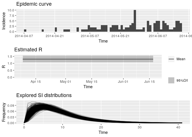
## TableGrob (3 x 1) "arrange": 3 grobs
## z cells name grob
## incid 1 (1-1,1-1) arrange gtable[layout]
## R 2 (2-2,1-1) arrange gtable[layout]
## SI 3 (3-3,1-1) arrange gtable[layout]
Look at the new median estimated R and 95%CrI: how different are they from your previous estimates? Do you think the size of the contacts dataset has had an impact on your results?
R_variableSI_median <- R_variableSI$R$`Median(R)`
R_variableSI_CrI <- c(R_variableSI$R$`Quantile.0.025(R)`, R_variableSI$R$`Quantile.0.975(R)`)
R_variableSI_median## [1] 1.296516
R_variableSI_CrI## [1] 1.078988 1.544788
Estimating time-varying transmissibility
When the assumption that ($R$) is constant over time becomes
untenable, an alternative is to estimating time-varying transmissibility
using the instantaneous reproduction number ($R_t$). This approach,
introduced by Cori et al. (2013), is also implemented in the package
EpiEstim. It estimates ($R_t$) for a custom time windows (default is
a succession of sliding time windows), using the same Poisson likelihood
described above. In the following, we estimate transmissibility for
1-week sliding time windows (the default of estimate_R):
config = make_config(list(mean_si = si_fit$mu, std_si = si_fit$sd))
# t_start and t_end are automatically set to estimate R over 1-week sliding windows by default. Rt <- # use estimate_R using method = "parametric_si"
# look at the most recent Rt estimates:
tail(Rt$R[, c("t_start", "t_end", "Median(R)",
"Quantile.0.025(R)", "Quantile.0.975(R)")])## Default config will estimate R on weekly sliding windows.
## To change this change the t_start and t_end arguments.
## t_start t_end Median(R) Quantile.0.025(R) Quantile.0.975(R)
## 60 61 67 1.2417304 0.8144152 1.797603
## 61 62 68 1.0045473 0.6318309 1.501326
## 62 63 69 0.8404935 0.5074962 1.294848
## 63 64 70 1.0276438 0.6538993 1.522464
## 64 65 71 1.0335607 0.6576643 1.531230
## 65 66 72 1.0337804 0.6578041 1.531556
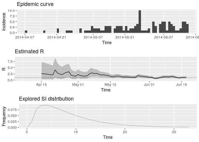
Plot the estimate of $R$ over
time:
plot(Rt, legend = FALSE)## Warning: Removed 1 rows containing missing values (geom_path).
## TableGrob (3 x 1) "arrange": 3 grobs
## z cells name grob
## incid 1 (1-1,1-1) arrange gtable[layout]
## R 2 (2-2,1-1) arrange gtable[layout]
## SI 3 (3-3,1-1) arrange gtable[layout]
How would you interpret this result? What is the caveat of this representation?
What would you have concluded if instead of using i_daily_trunc as
above, you ad used the entire epidemics curve io.e.
i_daily?
Rt_whole_incid <- # use estimate_R using method = "parametric_si",
# the same config as above but i_daily instead of i_daily_trunc
# look at the most recent Rt estimates:
tail(Rt_whole_incid$R[, c("t_start", "t_end",
"Median(R)", "Quantile.0.025(R)", "Quantile.0.975(R)")]) ## Default config will estimate R on weekly sliding windows.
## To change this change the t_start and t_end arguments.
## Warning in estimate_R_func(incid = incid, method = method, si_sample = si_sample, : You're estimating R too early in the epidemic to get the desired
## posterior CV.
## t_start t_end Median(R) Quantile.0.025(R) Quantile.0.975(R)
## 74 75 81 1.2330741 0.8412787 1.7310657
## 75 76 82 1.0008292 0.6564151 1.4488601
## 76 77 83 0.9432201 0.6128291 1.3753773
## 77 78 84 0.8202251 0.5158976 1.2258508
## 78 79 85 0.7452526 0.4566772 1.1356909
## 79 80 86 0.5146158 0.2811874 0.8515131
Save data and outputs
This is the end of part 2 of the practical. Before going on to part 3, you’ll need to save the following objects:
saveRDS(linelist, here("data/clean/linelist.rds"))
saveRDS(linelist_clean, here("data/clean/linelist_clean.rds"))
saveRDS(epi_contacts, here("data/clean/epi_contacts.rds"))
saveRDS(si, here("data/clean/si.rds"))